Normalizing Flows: Planar and Radial Flows

Simple distributions (e.g., Gaussian) are often used as likelihood distributions. However, the true distribution is often far from this simple distribution and this results in issues such as blurry reconstructions in the case of images. Latent variable models such as VAEs often set the prior distribution $p(\mathbf{z})$ to a factorial multivariate Gaussian distribution. Such a simplistic assumption hampers the model in multiple ways. For instance, this does not allow a multi-modal latent space distribution. Normalizing Flows allow transformation of samples from a simple distribution (subsequently denoted by $q_0$) to samples from a complex distribution by applying a series of invertible functions.

Distribution of a Simple Transformation of a RV

Before jumping into normalizing flows, let’s consider a simple univariate distribution $p(x)=2x$ with support $x\in[0,1]$. Define a function $y = f(x) = x^2$. Note that $f(x)$ is monotonically increasing in $[0,1]$. What is the PDF of the random variable $y$?

We can compute $p(y)$ using the CDFs as follows.

Now, $p(y) = F_{Y}’(y) = \frac{dF_{X}(\sqrt{y})}{dy}$ where

differentiating w.r.t. $y$ we get $\frac{d(y)}{dy} = 1$ which means that $p(y) = \mathcal{U}(0,1)$.

Change of Variables

The method described above can be extended to multivariate distributions $q_0(\mathbf{z})$ and smooth invertible mappings $f: \mathbb{R}^d\Rightarrow\mathbb{R}^d$. Samples $\mathbf{z} \sim q_0(\mathbf{z})$ can be transformed using $f$ to give $\mathbf{y}=f(\mathbf{z})$. The PDF of $\mathbf{y}$ is given by

where the second equality comes from the inverse-function theorem.

Rezende and Mohamed (2015) proposed two different families of invertible transformations: planar flow and radial flow.

Planar Flow

Planar flows use functions of form

where $\mathbf{u},\mathbf{w}\in \mathbb{R}^d$, $b \in \mathbb{R}$, and $h$ is an element-wise non-linearity such as $\tanh$.

The Jacobian is then given by

Now, using the matrix determinant lemma

Example

Let’s look at a specific example for $\mathbf{z}\in\mathbb{R}^2$. We will apply a planar flow to $\mathbf{z}$ to get $\mathbf{y} = f(\mathbf{z})$.

The determinant of the Jacobian can be computed using Eq. ($\ref{eq:planar-det}$) and the analytic PDF $q_1(\mathbf{y})$ can then be computed using Eq. ($\ref{eq:cov}$).

# Function to compute q0(z)
def mvn_pdf(X, mu=np.array([[0, 0]]), sig=np.array([[1, 0.], [0., 1]])):
    import numpy.linalg as LA
    sqrt_det_2pi_sig = np.sqrt(2 * np.pi * LA.det(sig))
    sig_inv = LA.inv(sig)
    X = X[:, None, :] - mu[None, :, :]
    return np.exp(-np.matmul(np.matmul(X, np.expand_dims(sig_inv, 0)),
                  (X.transpose(0, 2, 1))) / 2) / sqrt_det_2pi_sig

Let’s set up the required functions.

w = np.array([5., 0])
u = np.array([1., 0])
b = 0
def h(x):
    return np.tanh(x)
def h_prime(x):
    return 1 - np.tanh(x) ** 2
def f(z):
    y = z + np.dot(h(np.dot(z, w) + b).reshape(-1,1), u.reshape(1,-1))
    return y
def det_J(z):
    psi = h_prime(np.dot(z, w) + b).reshape(-1,1) * w
    det = np.abs(1 + np.dot(psi, u.reshape(-1,1)))
    return det

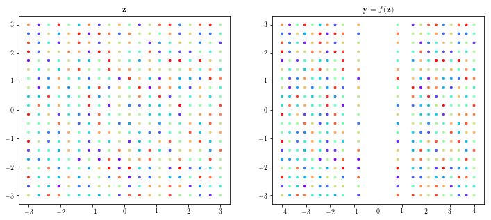
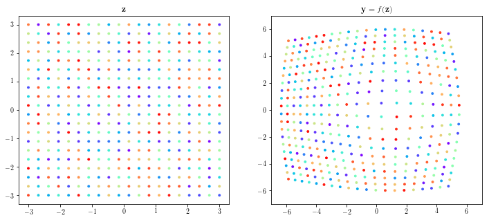
Let’s see how applying $f$ (Eq. $\ref{eq:planarfn}$) to points in a uniform grid moves them in the 2D space.

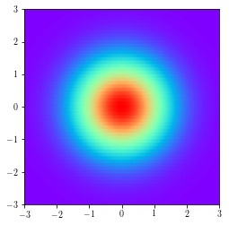
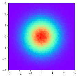
Let’s plot the analytic density $q_0(\mathbf{z})$ along with the empirical density by plotting a 2D histogram of samples from $q_0(\mathbf{z})$.

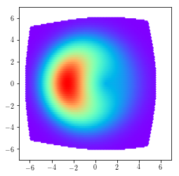
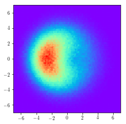
Now, let’s plot the analytic density $q_1(\mathbf{y})$ computed using Eq. (\ref{eq:cov}) along with the empirical density of $\mathbf{y}$.

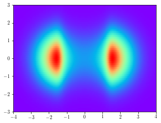
The analytic and empirical densities look similar. We’ve transformed a unimodal $q_0(\mathbf{z})$ into a bimodal $q_1(\mathbf{y})$ by applying a one level planar flow. Such functions can be successively applied multiple times to obtain a far more complex distribution.

Radial Flow

Radial flows use functions of the form

where $\alpha \in \mathbb{R}^+$, $\beta \in \mathbb{R}$, $h(\alpha,r) = (\alpha + r)^{-1}$ and $r = \vert\vert\mathbf{z} - \mathbf{z}_0\vert\vert$.

The Jacobian is then given by

Let $\gamma = (1+\beta h(\alpha,r))$. Again, using the matrix determinant lemma

Example

Let’s look at a specific example for $\mathbf{z}\in\mathbb{R}^2$. We will apply a radial flow to $\mathbf{z}$ to get $\mathbf{y} = f(\mathbf{z})$.

The determinant of the Jacobian can be computed using Eq. ($\ref{eq:radial-det}$) and the analytic PDF $q_1(\mathbf{y})$ can then be computed using Eq. ($\ref{eq:cov}$).

z0 = np.array([1, 0])
a = 2
b = 5
def h(r):
    return 1/(a+r)
def h_prime(r):
    return -1/(a+r) ** 2
def f(z):
    r = LA.norm(z - z0, axis=1).reshape(-1, 1)
    y = z + b * h(r) * (z - z0)
    return y
def det_J(z):
    n_dims = z.shape[1]
    r = LA.norm(z - z0, axis=1).reshape(-1, 1)
    tmp = 1 + b * h(r)
    det = (tmp + b * h_prime(r) * r) * tmp ** (n_dims - 1)
    return det

Let’s see how applying $f$ (Eq. $\ref{eq:radialfn}$) to points in a uniform grid moves them in the 2D space.

Let’s plot the analytic density $q_0(\mathbf{z})$ along with the empirical density by plotting a 2D histogram of samples from $q_0(\mathbf{z})$.

Finally, let’s plot the analytic density $q_1(\mathbf{y})$ computed using Eq. (\ref{eq:cov}) along with the empirical density of $\mathbf{y}$.

Not all functions of the forms given in Eqs. ($\ref{eq:planarfn}$) and ($\ref{eq:radialfn}$) are invertible. Some conditions need to be satisfied for them to be invertible. (See appendix in [1])

The complete code used in this post can be found in this repository.

References

[1] Rezende, D.J. and Mohamed, S., 2015. Variational inference with normalizing flows. arXiv preprint arXiv:1505.05770.
[2] Blog posts 1 and 2.