Monte Carlo Sampling using Langevin Dynamics

Langevin Monte Carlo is a class of Markov Chain Monte Carlo (MCMC) algorithms that generate samples from a probability distribution of interest (denoted by $\pi$) by simulating the Langevin Equation. The Langevin Equation is given by

\[\lambda\frac{dX_t}{dt} = -\frac{\partial V(x)}{\partial x} + \eta(t), \tag{1}\label{eq:langevin}\]

where $X_t$ is the position of a particle in a potential $V(x)$ and $\eta(t)$ is a noise term. The dynamics in Eq. ($\ref{eq:langevin}$) is also commonly written as the following Stochastic Differential Equation (SDE)

\[\mathrm{d}X_t = \underset{\text{drift term}}{\underbrace{-\nabla V(x)\mathrm{d}t}} + \underset{\text{diffusion term}}{\underbrace{\sqrt{2}\mathrm{d}B_t}} \tag{2}\label{eq:itodiff}\]

which represents an Itô diffusion, where $\mathrm{d}B_t$ denotes the time derivative of standard Brownian motion.

It can be shown that the SDE in Eq. ($\ref{eq:itodiff}$) has a unique invariant measure (or simply, a steady-state distribution) that does not change along the trajectory ($X_t$) of the particle. This means that if $X_0$ is distributed according to some probability density function $p_\infty$, then $X_t$ is also distributed according to $p_\infty$ for all $t \geq 0$. If we set the potential $V$ in Eq. ($\ref{eq:itodiff}$) cleverly such that $p_\infty = \pi$, then we can simulate the SDE (Eq. $\ref{eq:itodiff}$) to generate samples from $\pi$.

The steady-state distribution: choosing the potential

The Fokker-Plank equation is a partial differential equation (PDE) that describes the evolution of a probability distribution over time under the effect of drift forces and random (or noise) forces. The equivalent Fokker-Plank equation for the SDE in Eq. ($\ref{eq:itodiff}$) is given by

\[\frac{\partial p(x,t)}{\partial t} = \frac{\partial}{\partial x}\left[\frac{\partial V(x)}{\partial x}p(x,t)\right] + \frac{\partial^2p(x,t)}{\partial x^2}. \tag{3}\label{eq:fpe}\]

The steady-state solution of the Fokker-Plank equation is given by $\frac{\partial p(x,t)}{\partial t} = 0$. If $p_\infty$ is the steady-state distribution, we have

\[\frac{\partial p(x,t)}{\partial t} = \frac{\partial}{\partial x}\left[\frac{\partial V(x)}{\partial x}p_\infty(x) + \frac{\partial p_\infty(x)}{\partial x}\right] = \frac{\partial}{\partial x}J(x) = 0, \tag{4}\label{eq:steadystate}\]

where $J(x)$ denotes the probability “flux”. Eq. ($\ref{eq:steadystate}$) implies that $J(x)$ must be a constant; however, $p_\infty(x)$ and $\frac{\partial p_\infty(x)}{\partial x}$ must also satisfy certain boundary conditions. Specifically, the boundary condition that $J(x) = 0$ at infinity must be satisfied. Since $J(x) = 0$ at infinity and $J(x)$ is a constant, it must be equal to 0 everywhere. This leaves us with

\[J(x) = \frac{\partial V(x)}{\partial x}p_\infty(x) + \frac{\partial p_\infty(x)}{\partial x} = 0, \tag{5}\label{eq:zeroflux}\]

which has the solution

\[p_\infty(x) \propto \exp(-V(x)). \tag{6}\label{eq:gibbs}\]

Eq. ($\ref{eq:gibbs}$) represents a Gibbs distribution. This means that we can sample from energy-based models (EBMs) of the form $\pi(x) = \frac{\exp[-E(x)]}{Z}$, by setting $V(x) = E(x)$ in Eq. ($\ref{eq:itodiff}$). We can also write the distribution $\pi(x)$ as $\exp[\log\pi(x)]$, which means that we can set $V(x) = -\log\pi(x)$. It must be noted that we do not really need to know the normalization constant $Z$ for this to work because Eq. ($\ref{eq:itodiff}$) requires $\nabla\log\pi(x)$ and $\nabla Z = 0$ since $Z$ is a constant.

Simulating the SDE

Having derived the form of the potential $V(x)$, we are now interested in simulating the following SDE to sample from its steady state distribution, i.e., $\pi(x)$,

\[\mathrm{d}X_t = \nabla \log\pi(x)\mathrm{d}t + \sqrt{2}\mathrm{d}B_t. \tag{7}\label{eq:finalsde}\]

The SDE can be discretized using a numerical method such as the Euler-Maruyama method. The Euler-Maruyama approximation of Eq. ($\ref{eq:finalsde}$) can be written as

\[X_{t + \tau} - X_{t} = \tau\nabla \log\pi(x) + \sqrt{2}(B_{t+\tau}-B_{t}), \tag{8}\label{eq:eulerapprox1}\]

where $\tau$ is the step-size and $(B_{t+\tau}-B_{t}) \sim \mathcal{N}(0,\tau)$. This allows us to write Eq. ($\ref{eq:eulerapprox1}$) as

\[X_{t + \tau} = X_{t} + \tau\nabla \log\pi(x) + \sqrt{2\tau}\xi, \tag{9}\label{eq:eulerapprox2}\]

where $\xi \sim \mathcal{N}(0,1)$. The time-step $\tau$ can also be changed over time.

Unadjusted Langevin Algorithm

Eq. ($\ref{eq:eulerapprox2}$) gives us a method to sample from a probability distribution $\pi(x)$ by setting an initial seed $X_0$ and simulating the dynamics which, after a burn-in phase, will generate samples from $\pi(x)$. This algorithm is known as the Unadjusted Langevin Algorithm (ULA) which requires $\nabla \log\pi(x)$ to be $L$-Lipschitz for stability.

Metropolis-adjusted Langevin Algorithm

The ULA always accepts the new sample proposed by Eq. ($\ref{eq:eulerapprox2}$). Metropolis-adjusted Langevin Algorithm (MALA), on the other hand, uses the Metropolis-Hastings algorithm to accept or reject the proposed sample. Since $\xi \sim \mathcal{N}(0,1)$, $X_{t + \tau} \sim \mathcal{N}(X_{t} + \tau\nabla \log\pi(x),2\tau)$ in Eq. ($\ref{eq:eulerapprox2}$). This means that the proposal distribution is given by

\[q(x'|x) \propto \exp\left(-\frac{\|x'-x-\tau\nabla \log\pi(x)\|^2}{2\cdot2\tau}\right).\]

The sample ($\tilde{X}_{k+1}$) proposed by Eq. ($\ref{eq:eulerapprox2}$) is accepted with the following acceptance probability

\[\alpha := \min\left(1, \frac{\pi(\tilde{X}_{k+1})q(X_k|\tilde{X}_{k+1})}{\pi(X_{k})q(\tilde{X}_{k+1}|X_k)}\right).\]

Visualizing Langevin Monte Carlo Sampling

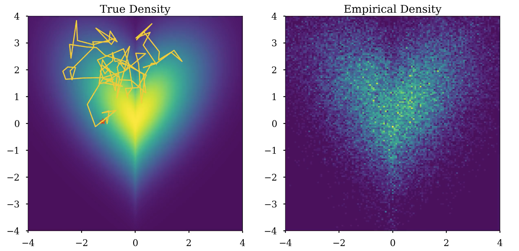
I set out to visualize these MCMC algorithms using matplotlib.animation to see how the distribution evolves over time. Unfortunately, writing to an MP4 file using matplotlib.animation is painfully slow and I could not find a simple way to speed it up. To solve this issue, I wrote a shell script to parallelize the generation of the chunks of the video and then combined them into one long video. The following video shows how samples are generated using MALA from a heart-shaped density given by

\[\pi(\mathbf{x}=\begin{bmatrix}x_1 & x_2\end{bmatrix}^\top) \propto \exp\left(-\frac{0.8x_1^2 + \left(x_2-\sqrt[3]{x_1^2}\right)^2}{2^2}\right).\]

The code used to generate the video above can be found here.

References

[1] Working with the Langevin and Fokker-Planck equations (notes).
[2] Chapter 4, Stochastic Processes and Applications, Grigorios A. Pavliotis (book).
[3] Wikipedia articles (a, b, c, d).