Implicit Reparameterization Gradients

Backpropagation through a stochastic node is an important problem in deep learning. The optimization of \(\mathbb{E}_{q_\phi(\mathbf{z})}[f(\mathbf{z})]\) requires computation of \(\nabla_\phi\mathbb{E}_{q_\phi(\mathbf{z})}[f(\mathbf{z})]\). Stochastic variational inference requires the computation of the gradient of one such expectation.

\(\definecolor{mBrown}{RGB}{188,99,16}\) \(\begin{align*} \mathcal{L}(\mathbf{x},\theta, \phi) = \color{mBrown}{\mathbb{E}_{q_{\phi}(\mathbf{z}|\mathbf{x})}[\log p_\theta(\mathbf{x}|\mathbf{z})]} - \color{black}\mathrm{KL}(q_{\phi}(\mathbf{z}|\mathbf{x})||p(\mathbf{z})) \end{align*}\)

Earlier methods of gradient computation include score-function-based estimators (REINFORCE) and pathwise gradient estimators (reparameterization trick). Recent works have proposed using reparametrizable surrograte distributions such as Gumbel-Softmax for Categorical, Kumaraswamy for Beta, etc. Other recent works such as Generalized Reparameterization Gradients (GRG) and Rejection Sampling Variational Inference (RSVI) have sought to build a generalized framework for gradient computation.

Explicit Reparameterization

It requires a standardization function \(\mathcal{S}_\phi(\mathbf{z})\) such that \(\mathcal{S}_\phi(\mathbf{z}) = \varepsilon \sim p(\varepsilon)\). It also requires \(\mathcal{S}_\phi(\mathbf{z})\) to be invertible. \(\mathbf{z}\sim q_\phi(\mathbf{z}) \Leftrightarrow \mathbf{z} = \mathcal{S}_\phi^{-1}(\varepsilon)\) and \(\varepsilon \sim p(\varepsilon)\).

\[\begin{align*} \nabla_\phi\mathbb{E}_{q_\phi(\mathbf{z})}[f(\mathbf{z})] &= \mathbb{E}_{q(\varepsilon)}[\nabla_\phi f(\mathcal{S}_\phi^{-1}(\varepsilon))]\\ &= \mathbb{E}_{q(\varepsilon)}[\nabla_\mathbf{z}f(\mathcal{S}_\phi^{-1}(\varepsilon))\nabla_\phi\mathcal{S}_\phi^{-1}(\varepsilon)] \end{align*}\]

Implicit Reparameterization

Implicit Reparameterization eliminates the restrictive requirement of an invertible \(\mathcal{S}_\phi(\mathbf{z})\).

\[\begin{align} \nabla_\phi\mathbb{E}_{q_\phi(\mathbf{z})}[f(\mathbf{z})] &= \mathbb{E}_{q(\varepsilon)}[\nabla_\mathbf{z}f(\mathcal{S}_\phi^{-1}(\varepsilon))\nabla_\phi\mathcal{S}_\phi^{-1}(\varepsilon)]\\ &=\mathbb{E}_{q_\phi(\mathbf{z})}[\nabla_\mathbf{z}f(\mathbf{z})\nabla_\phi\mathbf{z}] \end{align}\] \[\begin{align} \frac{d\mathcal{S}_\phi(\mathbf{z})}{d\phi} = \frac{d\varepsilon}{d\phi} &= 0\tag{1}\\ \frac{\partial\mathcal{S}_\phi(\mathbf{z})}{\partial\mathbf{z}}\frac{d\mathbf{z}}{d\phi} + \frac{\partial\mathcal{S}_\phi(\mathbf{z})}{\partial\phi} &= 0\tag{2} \end{align}\] \[\begin{align} \nabla_\phi\mathbf{z} = -(\nabla_\mathbf{z}\mathcal{S}_\phi(\mathbf{z}))^{-1}\nabla_\phi\mathcal{S}_\phi(\mathbf{z}) \end{align}\]

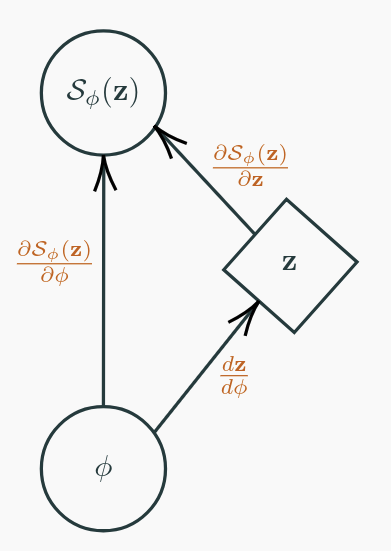
where Eq. (1) uses the fact that the total derivative of noise with respect to the distribution parameters is 0 and Eq. (2) applies the multivariate chain rule based on Figure 1.

Examples

Normal Distribution

The standardization function for the normal distribution is \(\mathcal{S}_\phi(\mathbf{z}) = \frac{\mathbf{z}-\mu}{\sigma} \sim \mathcal{N}(\mathbf{0},\mathbf{I})\).

• Explicit Reparameterization: \(\mathcal{S}_\phi^{-1}(\varepsilon) = \mu + \sigma\varepsilon \Rightarrow \frac{d\mathbf{z}}{d\mu} = 1\) and \(\frac{d\mathbf{z}}{d\sigma} = \varepsilon\).
• Implicit Reparameterization: \(\frac{d\mathbf{z}}{d\mu} = -\frac{d\mathcal{S}_\phi(\mathbf{z})/d\mu}{d\mathcal{S}_\phi(\mathbf{z})/d\mathbf{z}} = 1\) and \(\frac{d\mathbf{z}}{d\sigma} = -\frac{d\mathcal{S}_\phi(\mathbf{z})/d\sigma}{d\mathcal{S}_\phi(\mathbf{z})/d\mathbf{z}} = \frac{\mathbf{z}-\mu}{\sigma}\).

Using Cumulative Distribution Function

The CDF can be used as a standardization function by using the property that for a random variable \(\mathbf{z}\), the random variable \(\mathbf{y} = F_\phi(\mathbf{z})\) has the uniform distribution on \([0,1]\) where \(F_\phi\) is the CDF. The gradient can then be computed as follows.

\[\nabla_\phi\mathbf{z} = -\frac{\nabla_\phi F_\phi(\mathbf{z})}{q_\phi(\mathbf{z})}\]

Conclusion

Implicit Reparameterization allows stochastic backpropagation through a variety of distributions such as truncated, mixtures, gamma, Von-Mises, Beta, etc. Check out these slides and the paper.

References

[1] Figurnov, M., Mohamed, S. and Mnih, A., 2018. Implicit Reparameterization Gradients. arXiv preprint arXiv:1805.08498.
[2] Jang, E., Gu, S. and Poole, B., 2016. Categorical reparameterization with gumbel-softmax. arXiv preprint arXiv:1611.01144.
[3] Kingma, D.P. and Welling, M., 2013. Auto-encoding variational bayes. arXiv preprint arXiv:1312.6114.
[4] Naesseth, C.A., Ruiz, F.J., Linderman, S.W. and Blei, D.M., 2016. Reparameterization gradients through acceptance-rejection sampling algorithms. arXiv preprint arXiv:1610.05683.
[5] Ruiz, F.R., AUEB, M.T.R. and Blei, D., 2016. The generalized reparameterization gradient. In Advances in neural information processing systems (pp. 460-468).